Step 1 : Mosaic
The 9 raster tiles are assembled using the Mosaicking tool.
Tools tab <> Tools Libraries <> Grid <> Tools <> Mosaicking
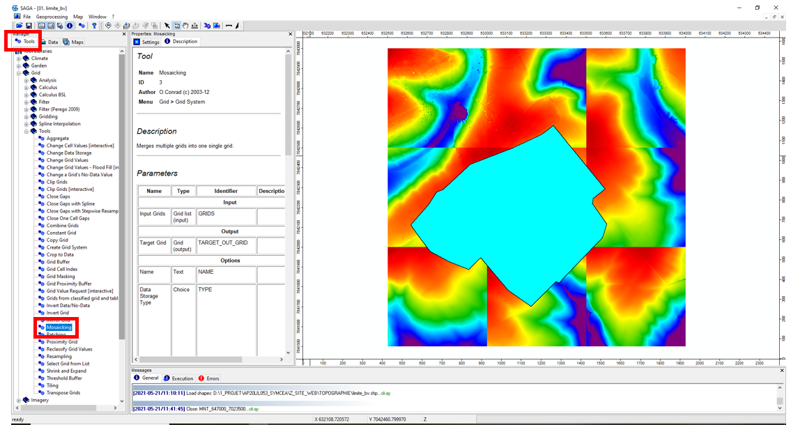
Double-click on Mosaicking to launch the tool. Click on Input Grids, then on Parcourir (Browse) (3 dots left). Import all tiles with the Flèche (Arrow) >. Click on OK.
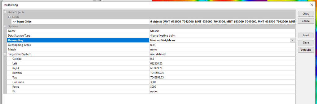
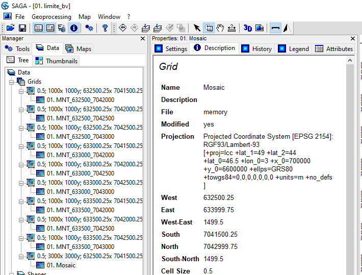
The Mosaicking tool then displays the new Grid System of the new DTM resulting from the assembly of the 9 tiles. By default, the proposed resolution is that of the input tiles, i.e. 0.5 m. The new DTM is 3000 rows by 3000 columns. The Lambert 93 coordinates of the corners (Left, Right, Bottom, Top) are also specified. Click on OK. The new DTM appears in the Data tab under the name Mosaic.

Note : MNT stands for « Modèle Numérique de Terrain » which is the French equivalent for DTM « Digital Terrain Model ».
This tool also lets you modify the resolution of the output DTM by resampling. Simply change the Cellsize value and select a resampling method. In order to demonstrate SAGA’s numerous tools, the DTM is resampled in the remainder of this tutorial using the dedicated Resampling tool. Resampling is not always necessary and depends on the modeling objectives.
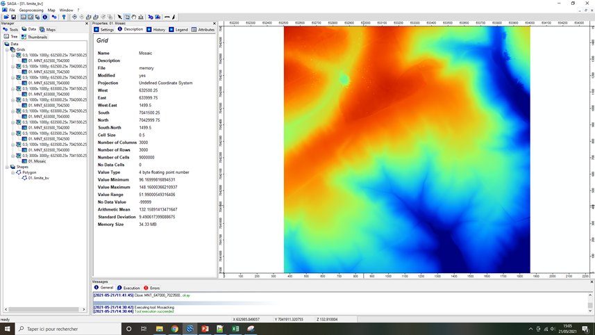
To view the new DTM, right-click on Mosaic, Add to Map, Select the limite_bv map and click OK.
Step 2 : Definition of a projection system
By clicking on the Description tab, Mosaic does not have a projection system (Undefined Coordinate System).

The Set Coordinate Reference System tool is used to define a projection system for a shape or grid.
Tools tab <> Tools Libraries <> Projection <> Proj.4 <> Set Coordinate Reference Sytem
Double-click on Set Coordinate Reference System to launch the tool. Click on Grids, then on Parcourir (Browse) and load Mosaic. Each projection system is defined by an EPSG code. By default, the tool proposes EPSG code 4326, which corresponds to WGS84 (world geodetic system). Replace code 4326 with the EPSG code for the Lambert 93 projection system (2154). Click on OK.

Click on Mosaic, then on the Description tab. The projection system is replaced by RGF/Lambert 93.
Optional : Resampling
This step is optional but mandatory for this tutorial!
The lower the DTM resolution used, the longer the calculation times. The idea is therefore to adapt the DTM resolution to the desired level of detail. Typically, resolutions between 1 and 5 m are the ones most often used with the WaterSed model (optimal compromise between computation time and digital landscape description).
In this tutorial, we’ll use the SAGA GIS Resampling tool to aggregate values from 0.5 m to 1 m resolution.
Tools tab <> Tools Libraries <> Grid <> Tools <> Resampling
Select the Grid System of the Mosaic grid. Click on Grids and load Mosaic. In our example, the resolution (Cellsize) is increased to 1 m. This reduces the number of rows and columns from 3000 to 1500. The default resampling method (Upscaling method) is Mean Value, i.e. an average of the altitude values. Click on OK.

The new DTM appears in the Data tab under the name Mosaic with the new Grid System.

At this point, save Mosaic. Right-click on Mosaic, Save as… In this example, the Mosaic grid is saved as mnt_brut in the :
/TUTORIEL/PREPROCESSING/TOPOGRAPHIE/mnt_brut.sgrdDelete the 9 tiles used to build Mosaic. To delete a tile, Right-click, Close.
Optional : DTM hillshading
This step is optional but mandatory for this tutorial!
Shading is used to obtain the hypothetical illumination of a surface by determining the illumination values of each raster cell. This method defines the position of a hypothetical light source and calculates the illumination values of each cell in relation to neighboring cells. Shading significantly improves the visualization of a DTM.
In SAGA GIS, DTM shading is performed using the Analytical Hillshading tool.
Tools tab <> Tools Libraries <> Terrain Analysis <> Lighting, Visibility <> Analytical Hillshading
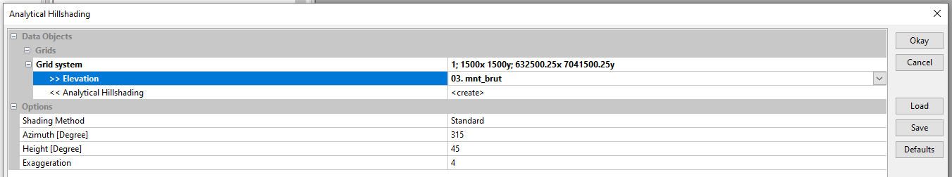
Select the Grid System of the mnt_brut grid. Click on Elevation and load mnt_brut. Use the various options to adjust the grid lighting. Leave the default options. Click on OK.
The shading grid appears in the Data tab under the name Analytical Hillshading. To view Analytical Hillshading, right-click on Analytical Hillshading , Add to Map, select the limite_bv map and click OK.

Save Analytical Hillshading. Right-click on Analytical Hillshading , Save as… In this example, the Analytical Hillshading grid is saved as hillshade.
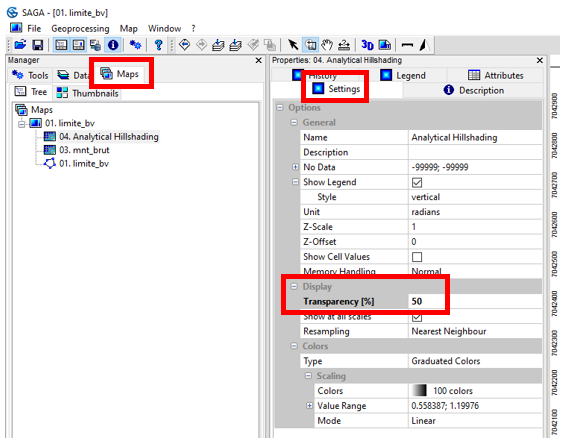
/TUTORIEL/PREPROCESSING/TOPOGRAPHIE/hillshade.sgrdThe color gradient of DTM heights (red – yellow – blue) can be added by adjusting the transparency of the Analytical Hillshading grid.
In the Maps tab, check the order of the different layers displayed in the limite_bv map. Analytical Hillshading should be in first position and mnt_brut in second position. Click on Analytical Hillshading then go to the Settings tab. In the Display menu, replace the 0% Tranparency (%) value by 50% and click on Apply.