Quick Start

1. Launch

The WaterSed model is running from the SAGA GIS software. SAGA GIS (System for Automated Geoscientific Analyses) is an open source, multi-platform geographic information system (GIS) software released under the GPL licence.

1.1 Setting up SAGA-GIS

Download and set-up the latest SAGA-GIS version :

https://sourceforge.net/projects/saga-gis/files/

As of 30/09/2021, the latest version of SAGA is 8.0.1 Go to the SAGA – 8 directory and then to the SAGA – 8.0.1 directory. Various SAGA GIS formats are available

>> If you have administrator rights on your PC to install a software, download saga-8.0.1_x64_setup.exe. Run this setup program and install SAGA-GIS. Launch SAGA-GIS from the icon on your desktop.

>>If you do NOT have administrator rights, SAGA-GIS offers a portable version. Download saga-8.0.1_x64.zip and unzip the file in the directory of your choice. Open the directory and launch SAGA-GIS by double-clicking on saga_gui.

Note: If your version of Windows is 32-bit, simply download saga-8.0.1_win32_setup.exe or saga-8.0.1_win32.zip depending on your administrator rights.

When SAGA-GIS is launched, various windows appear. You can stretch the left-hand windows for better visibility.

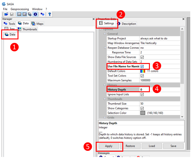
SAGA-GIS needs to be configured the first time it is launched. Click on Data (1), then click on Settings (2) and tick Use file name for naming (3). Replace the -1 value for History Depth with 0 (4). Click on Apply (5).

1.2 WaterSed setup

Download the WaterSed model from the site’s Download tab (after filling in the download request form, you will be automatically redirected to the model download page). The WaterSed model comes in the form of an .xml toolchain named WATERSED_v3.0.xml.

Drag and drop WATERSED_v3.0.xml into the Tools window. The WaterSed model is then automatically installed in SAGA GIS. To install the other WaterSed tools, drag and drop them as well.

The model appears in the Tools tab. The Tools tab contains all the SAGA GIS tools. To discover the different tools, simply unfold the drop-down menus using the (+) button. The WaterSed model is located in the Tool Chains menu, WaterSed.

To launch the Watersed model, double-click on WaterSed Model. The model window will appear.

2. Interface description

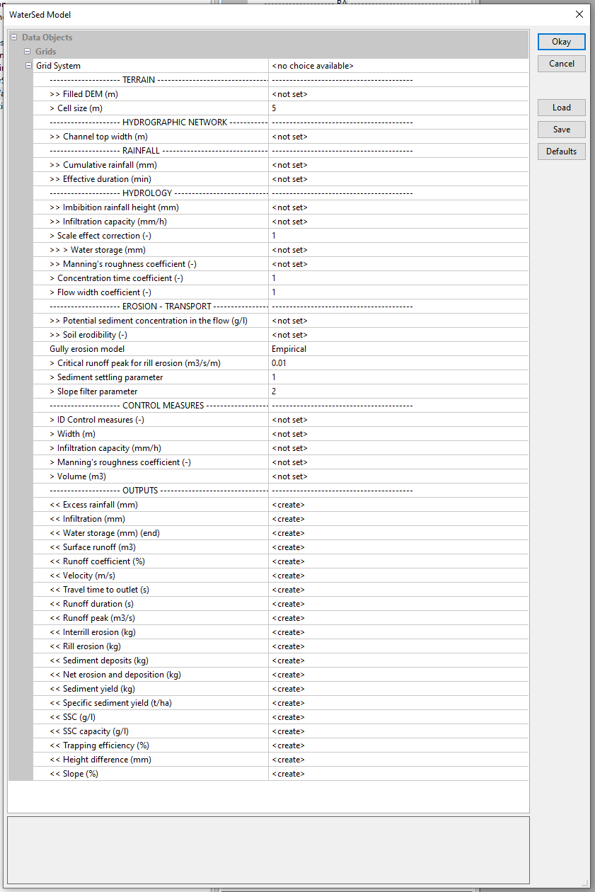
The model interface is organised into menus. The input data is divided into 6 different menus: TERRAIN, HYDROGRAPHIC NETWORK, RAINFALL, HYDROLOGY, EROSION – TRANSPORT and CONTROL MEASURES (optional). The model’s output grids are grouped in the OUTPUTS menu.

Modelling is carried out on a study area defined according to a Grid System. Once the Grid System has been filled in, 10 grids are required to run the WaterSed model. Once the grids have been filled in, click on OK to run the model.

TERRAIN Menu

Filled DEM (m) : Digital Terrain Model (DTM) with hydrological correction
Cell size (m) : DTM resolution

HYDROGRAPHIC NETWORK Menu

Channel top width (m) : full width of watercourses (value 0 outside watercourses)

RAINFALL Menu

Cumulative rainfall (mm) : total rainfall height
Effective time (min) : effective duration of the event

HYDROLOGY Menu

Imbibition rainfall height (mm) : initial loss before runoff appears; imbibition is a function of soil texture and structure as well as initial soil moisture ;
Infiltration capacity (mm/h) : infiltration rate if the soil is saturated and homogeneous (continuous loss); this infiltration rate particularly depends on the texture and structure of the soil;
Scale effect correction (-) : parameter used to adjust soil infiltrability (between 0 and 1).
Water storage (mm) : maximum height of water to fill the soil porosity; a function of soil thickness and porosity;
Manning’s roughness coefficient (-) : coefficient reflecting the forces of friction on the soil surface, as a function of soil roughness and vegetation cover;
Concentration time coefficient (-) : concentration time contraction/dilation factor (between 0.5 and 1.5).
Flow width coefficient (-) : flow flooding rate (between 0 and 1). A value of 1 indicates that 100% of the mesh width is flooded. This value is modified when the DTM resolution is high (greater than 25 m).

EROSION-TRANSPORT Menu

Potential sediment concentration in the flow (g/l) : concentration of suspended solids in runoff water (g/l); sensitivity of the soil to detachment under the action of rain (« splash effect »)
Soil erodibility (-) : soil erodibility (value between 0 and 1); sensitivity of the soil to detachment under the action of runoff.
Gully erosion model : choice of concentrated erosion module (« Empirical » or « KSV »); see the Theory tab for details of each module
Critical runoff peak for rill erosion (m³/m/s) : specific flow threshold triggering concentrated erosion
Sediment settling parameter (-) : parameter used in the transport capacity equation to regulate sediment settling.
Slope parameter (-) : parameter used to adjust the effect of slope on sediment deposition

CONTROL MEASURES Menu

ID Control measures (-) : Identifier characterising the type of layout: (1) Fascine, (2) Hedge, (3) Grassed strip, (4) Pond / Basin
Width (m) : cross-sectional width of the layout
Infiltration capacity (mm/h) : infiltration capacity of the layout
Manning (s.m^-1/3) : Manning’s roughness coefficient
Volume (m3) : storage volume

OUTPUTS Menu

Excess rainfall (mm) : net rainfall
Infiltration (mm) : total height of rainfall and infiltrated runoff
Water storage end (mm) : soil water storage capacity at the end of the event
Surface runoff (m³) : total volume of runoff discharged during the event
Runoff coefficient (%) : ratio between runoff volume and rainfall volume
Velocity (m/s) : water flow speed
Travel time to outlet (s) : time taken for water to travel to the catchment outlet
Runoff duration (s) : runoff duration
Runoff peak (m³/s) : runoff peak
Interrill erosion (kg) : raw erosion due to the action of rain (diffuse erosion)
Rill erosion (kg) : raw erosion due to runoff (concentrated erosion)
Sediment deposits (kg) : raw deposits of sediment
Net erosion and deposition (kg) : balance between raw erosion and raw deposition
Sediment yield (kg) : sediment flow or total quantity of sediment transported during the event
Specific sediment yield (t/ha) : ratio between sediment flow and drained area
SSC (g/l) : concentration of suspended solids in run-off water
SSC capacity (g/l) : concentration of SPM in runoff water at transport capacity
Trapping efficiency (%) : sediment deposition rate (input-output balance)
Height difference (mm) : net erosion and deposition expressed in mm
Slope (%) : local slope

3. First run

Download the dataset : here

Unzip the file first_run_watersed.zip into the directory of your choice. The dataset contains 10 raster grids in SAGA GIS format (.sgrd).

Launch SAGA GIS. The software is organised into windows, each with a specific function. You can change the way the windows are displayed using the Window menu.

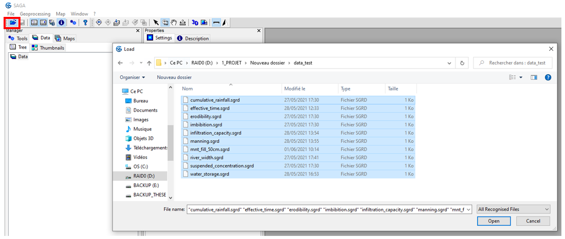
To import the raster grids, click Open and point to the directory. Select the 10 .sgrd files. Click on Open.

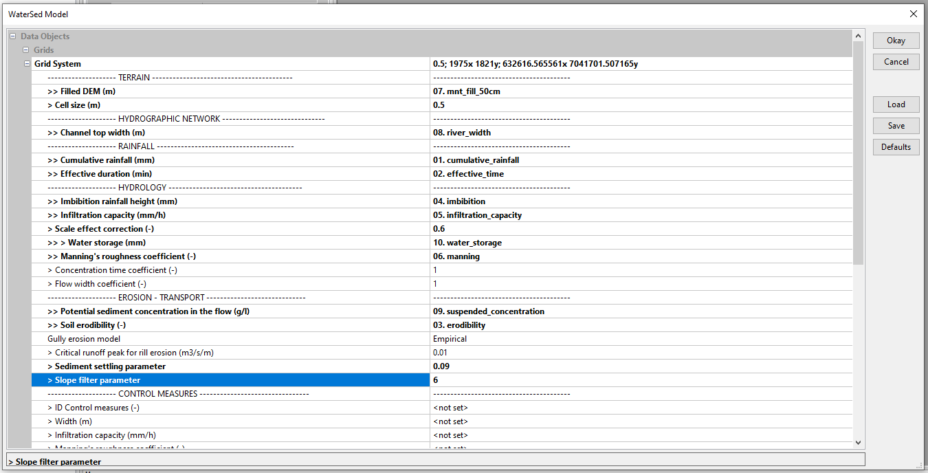
Raster grids are automatically loaded in the Data, Grids tab. In SAGA GIS, each raster tile is classified according to its Grid System. The Grid System describes the resolution of the tile (0.5), the number of rows and columns (1975x; 1821y) and the X and Y coordinates of the bottom left corner of the tile (632616.565561x 7041701.507165y) (in Lambert 93).

Launch the WaterSed model. Load the various raster grids. Change the default model parameters to the following values :

Cell size (m) : 0.5
Scale effect correction (-) : 0.6
Concentration time coefficient (-) : 1
Flow width coefficient (-) : 1
Gully erosion model : Empirical
Critical runoff peak for rill erosion (m3/m/s) : 0.01
Sediment settling parameter (-) : 0.09
Slope parameter : 6

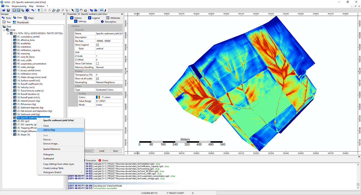
Click on Okay. At the end of the simulation, the model outputs appear in the Data, Grids tab, under the input raster grids. To display a raster grid, Right-click on the grid, Add to Map.

Viewing / Navigation

To move the raster grid, select the Hand button. To zoom in and out, select the Zoom button.

To get a cell value, zoom in using the zoom button until the mesh is visible. Go to the Data tab. Highlight the raster grid you want to query (Specific Sediment Yield in our example). Go to the Attributes tab. Select the Action button. Click on a cell. The selected cell is surrounded by a red square. The value of the mesh appears in the Attributes tab.